Waterfowl at your service: How ducks and geese help our environment

Waterfowl and waterbirds are integral parts of wetland ecosystems. Ducks, geese and other migratory birds deliver more valuable benefits to our environment and to us than we realize.

By Lauren Rae May 22, 2020

Wood duck

As dedicated conservationists, we’re committed to ensuring that waterfowl have the habitats they need to thrive. But what have they done for us, lately? Turns out, it’s a whole lot.


Many of us get unspeakable joy from being near a local wetland at sunset as flocks of birds return from an evening of feeding. Others treasure the family tradition of setting up a blind in the marsh on a brisk autumn morning.

After decades of successful conservation work spanning North America, waterfowl populations are strong, bringing with them endless opportunities for us to enjoy their beauty and bounty.

But there’s more to appreciate about our feathered friends than you may realize. As ambassadors for the ducks, we feel compelled to highlight some of the lesser known and unique services they provide. Allow us to sing (quack and honk) their praises.

Hen with brood
Hen with brood © Brendan Kelly

Waterfowl help biodiversity with wetland-to-wetland delivery

Waterfowl and waterbirds are integral parts of wetland ecosystems. They’re large-bodied and often airborne, which makes them relatively easy to observe. And they’re mobile; travelling far distances and stopping at multiple wetland sites along the way. Every time they splash down at these migratory pit stops, they leave something behind, like an avian Amazon delivery driver.

Last year, DUC restored more than 50,000 acres (20,200 hectares) of wetlands. When waterfowl visit these newly restored habitats, they can establish biodiversity by introducing plant, invertebrate, amphibian and fish species from other sites. Frog eggs might get transported from pond to pond if they are stuck on a goose’s foot, for example. Insect larvae that survive in a duck’s intestinal tract might get deposited in a wetland far from where it was ingested.

This wetland-to-wetland delivery method works for established ecosystems, too. In the face of climate change, dispersal by waterbirds can help a species shift its range. As conditions get warmer, waterfowl can help other species expand northward to climates where they can continue to be successful. It also helps keep a species’ gene pool diverse, making it easier for the species to avoid inbreeding and adapt to changing environments. Having many types of genes gives species a stronger toolkit for facing adversity. Either way, dispersal by waterbirds can benefit individual species and enhance biodiversity in wetlands.

Scaup
Scaup © Greg Schneider

How birds help with pest problems and invasive species

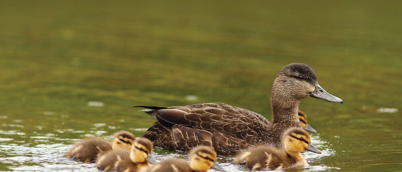
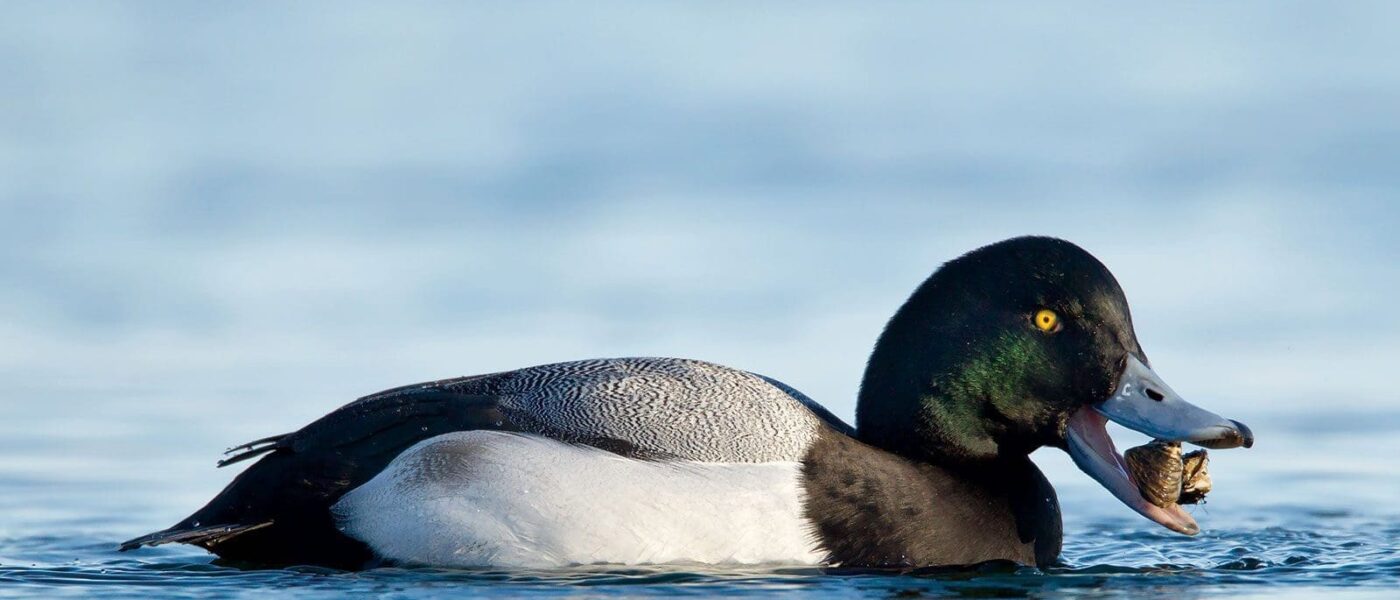
Introduced or invasive species often raise a red flag—and rightfully so. They wreak havoc on natural ecosystems and have major economic consequences. Although they could potentially spread undesirable species to new areas, waterfowl can be of help here, too. For instance, diving ducks like scaup feed on invasive zebra mussels and can decrease their abundance. The same holds true for plant pests. Ducks that winter in flooded rice fields eat the seeds of weeds, giving the farmer a leg-up the following growing season. Ducklings, too, can make a dent in pest populations. They eat a lot of larvae that would otherwise become pesky, biting mosquitoes.

Canada goose
Canada goose © Chantal Jacques

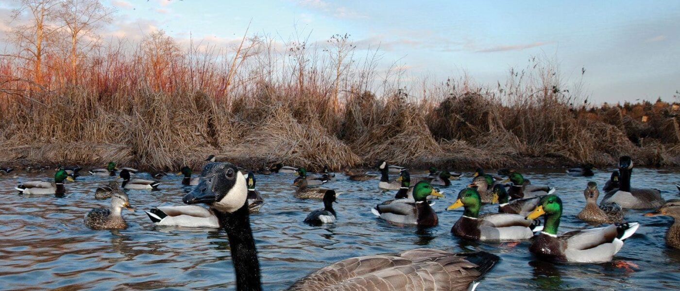
Security detail provided by Canada geese

Canada geese are notorious for protecting their nests and goslings during the breeding season. This aggression can benefit other birds nesting nearby, keeping predators—and people—at a safe distance, which helps survival of young birds regardless of their species.

Waterfowl help ecosystems and the economy

Anyone that has a hard time appreciating the many ways waterfowl help ecosystems should know that they contribute financially, too. With all that hunters invest in waterfowling, a single duck is worth $26 in the Canadian economy (not to mention that northern communities have traditionally subsisted on waterfowl harvest and it continues to be a cornerstone of many cultures). And in Iceland, one of the last remaining locations where down from non-domesticated ducks is harvested, eider feathers bring $40 million to retail markets.

The ripple effect of conservation

It’s comforting to know that, whatever our reasons for conserving wetlands, our work on behalf of the ducks supports hundreds of other species, including ourselves.

Where have all the wetlands gone?

Peter, Paul, and Mary could very easily have been talking about our country’s wetlands instead of flowers in their 1962 hit, “Where Have All the Flowers Gone.”  When wetlands were first forming, thousands of years ago as the ice age ended, the United States was 90% covered with wetlands. Today, coastal and inland wetlands cover only about 5.5% of the United States. 

The Ramsar Convention estimates that nearly 90 percent of all the world’s wetlands have disappeared since the 1700s, and those that remain are at risk of disappearing three times faster than forests. In 1989, Congress directed the Department of the Interior to compare the estimated total number of wetland acres in the 1780s and in the 1980s in the areas that now comprise each state. The report, released by the U.S. Fish and Wildlife Service (FWS), was designed as a one-time effort to document historical wetland losses from colonial times through the 1980s. This report is updated every 10 years providing new information based on a statistical analysis of wetlands changes from the 1970s through the 1980s.

As with historical estimates, data on present wetland acreage must be interpreted with caution. For some states, wetlands have been mapped for the entire state by the FWS National Wetlands Inventory. However, for those states where wetlands are not completely mapped or where acreage summaries are not yet compiled, an accurate accounting of wetland acreage is not always available, so the best national or regional data available to determine statewide totals was used. Additionally, the status of wetlands in the United States is constantly changing. It is estimated that, on average , over 60 acres of wetlands have been lost every hour in the lower 48 states during this 200-year time span.

Considerable changes in wetland distribution and abundance have taken place since the 1780s. In the conterminous United States, only an estimated 104 million acres of wetlands remained through the 1980s, representing a 53-percent loss from the original acreage total. If Alaska and Hawaii are counted, an estimated 274 million wetland acres remain.

By all estimates, the national decline in wetlands from the 1780s to the 1980s is dramatic. Losses in particular regions of the country such as the mid-western farm belt states of Illinois, Indiana, Iowa, Michigan, Minnesota, Ohio, and Wisconsin are even more startling. Alaska stands alone as the only state in which wetland resources have not been substantially reduced. 

Incomplete baseline data on the wetlands in the United States prevents an accurate appraisal of the “health” of these remaining resources. However, population growth and distribution and agricultural development greatly affect land-use patterns that impact wetlands . Despite increased efforts to conserve wetlands through state and federal legislation, hundreds of thousands of acres have been drained annually. Wetland acreage has diminished to the point where environmental and even socio-economic benefits are now seriously threatened.

The years from the mid-1950s to the mid-1970s were a time of major wetland loss, but since then the rate of loss has decreased. How will climate change and global warming affect wetlands as our country and the rest of the world continue to experience unprecedented heat waves. The fact that the definition of a wetland changes often makes these numbers even harder to predict. The total amount of wetlands can change in an instant depending on the wording of a government document. 

Various factors have contributed to the decline in the loss rate of wetlands including implementation and enforcement of wetland protection measures and elimination of some incentives for wetland drainage. Public education and outreach about the value and functions of wetlands, private land initiatives, coastal monitoring and protection programs, and wetland restoration and creation actions have also helped reduce overall wetland losses.  Hopefully, this will be enough.

References:

https://share.america.gov/us-protects-wetlands/
https://www.archives.gov/

https://georgewbush-whitehouse.archives.gov › 2004/04

The Wetlands Initiative; Founded, 1994,  http://www.wetlands-initiative.org/


How the U.S. Protects the Environment, From Nixon to Trump By Robinson Meyer

Dahl, T.E. and C.E. Johnson . 1991. Status and Trends of Wetlands in the

Conterminous United States, Mid-1780’s to Mid-1980’s. U.S. Department of

the Interior, Fish and Wildlife Service, Washington, D.C.

The Kissimmee River Restoration Project

Only about one-half of Florida’s original wetlands remain, but Florida still has more wetlands than any of the other forty-seven conterminous States. On top of that, over the last few decades, the State of Florida has been diligently restoring some of the lost wetlands.

The Kissimmee River once meandered for 103 miles through central Florida. Its floodplain, reaching up to three miles wide, was inundated for extended periods by heavy seasonal rains. Native wetland plants, wading birds and fish thrived there. The Kissimmee Basin encompasses more than two dozen lakes in the Kissimmee Chain of Lakes (KCOL), their tributary streams and associated marshes and the Kissimmee River and floodplain. The basin forms the headwaters of Lake Okeechobee and the Everglades; together they comprise the Kissimmee-Okeechobee-Everglades (KOE) system, but prolonged flooding in 1947 prompted a public outcry for federal assistance to reduce flood damage to property. In 1948, the U.S. Congress authorized the U.S. Army Corps of Engineers to construct the Central and South Florida Project.

Site History

In the 1960s, the Central and Southern Florida Flood Control (C&SF) Project modified the native KOE system extensively throughout South Florida, including construction of canals and water control structures to achieve flood control in the Upper and Lower Kissimmee basins. The Kissimmee River was channelized by cutting and dredging a 30-feet-deep straightaway through the river’s meanders creating the C-38 canal.

After the river channel was straightened, 40,000 acres of floodplain below Lake Kissimmee dried out, reducing the quality of waterfowl habitat by ninety percent, and the number of herons, egrets and wood storks by two-thirds. Catches of largemouth bass in the river were consistently worse after the channelization. While the Kissimmee was not a significant source of pollution for Lake Okeechobee before channelization, in the 1970s and later the river contributed about 25% of the nitrogen and 20% of the phosphorus flowing into the lake.

While the project delivered on the promise of flood protection, it also destroyed much of a floodplain-dependent ecosystem that nurtured threatened and endangered species, as well as hundreds of other native fish and wetland-dependent animals.

Efforts to restore the Kissimmee River to its original flow were approved by Congress in 1992 and began with modification to the headwater lakes in 1997. The United States Army Corps of Engineers had initially hoped to complete the project in 2015. In 2006, the South Florida Water Management District had acquired enough land along the river and in the upper chain of lakes to complete restoration. In all, forty-three miles (69 km) of the Kissimmee River will be restored.

Project Goals

Major initiatives in the Kissimmee Basin include the Kissimmee River Restoration Project, the Kissimmee River Restoration Evaluation Program and the Kissimmee Chain of Lakes and Kissimmee Upper Basin Monitoring and Assessment. Several activities are associated with these projects, including ecosystem restoration, evaluation of restoration efforts, aquatic plant management, land management, water quality improvement and water supply planning.

The Kissimmee River Restoration Project will restore more than forty square miles of the river floodplain ecosystem, 20,000 acres of wetlands, and forty-four miles of the historic river channel. This major restoration effort is a 50-50 partnership between the USACE and the SFWMD. Over the past 22 years, the USACE and SFWMD worked together to:

  • Complete backfilling of 22-miles of the C-38 canal between Lakes Kissimmee and Okeechobee.
  • Reconstruct remnant river channels across the backfilled canal to reconnect and restore flow in remnant river channels.
  • Remove two water control structures.
  • Add two gates to the S-65 water control structure.
  • Acquire more than 100,000 acres of land to restore the river and floodplain.

Restoration Progress

Already, wildlife is returning to the restored sections of the river. When flooding began again, muck and smothering aquatic weeds were flushed out. Sandbars reemerged. Encroaching dry land trees began dying back. Once-dormant plants began to reestablish themselves. The species included pink-tipped smartweed, horsetail, sedges, rushes, arrowhead, duck potato and pickerel weed. Flooding and continuous flow increased levels of dissolved oxygen in the water, creating near perfect conditions for aquatic invertebrates such as insects, mollusks, works, crayfish, and freshwater shrimp. This, in turn, boosted fish populations and it led to a rise in bird and alligator populations. The entire food chain benefited. The Kissimmee River restoration is one of the largest ecosystem restoration projects in the world.

The decades-long project to restore the historic Kissimmee River is now nearing completion. There’s two phases to complete Kissimmee River restoration,” said Lawrence Glenn, director of the SFWMD’s water resources division. “The first step, construction, is now complete. Next is what Glenn calls “the restoration of hydrology.” 

Standing from the bow of an airboat, Glenn pointed to the meandering grassy waters behind him. In the exact spot where the C-38 Canal once flowed, there was now an abundance of birds flying overhead. “The next step is managing the quantity, timing and distribution of the river’s water, to ensure the ecology thrives,” he said. 

Sources

Chesnes, M. (2021). ‘A fantastic day’: Kissimmee River restoration project complete after 22 years. TCPalm. Retrieved from https://www.tcpalm.com/story/news/local/indian-river-lagoon/2021/07/29/army-corps-kissimmee-river-restoration-project-complete-22-years-lake-okeechobee-releases-discharges/5399944001/

Koebel Jr., J. W. (1995). An historical perspective on the Kissimmee River restoration project. Restoration Ecology, 3(3), Pages 149-159. Retrieved from https://doi.org/10.1111/j.1526-100X.1995.tb00167.x

South Florida Management District. (n.d.). Kissimmee River. Retrieved from https://www.sfwmd.gov/our-work/kissimmee-river

Biological Control of Purple Loosestrife

John D. Byrd, Mississippi State University, Bugwood.org

Introduced species that cause economic or environmental harm, or harm to human health, are called invasive species. The National Invasive Species Information Center states that “…these plants are characteristically adaptable to new habitats, grow aggressively, and have a high reproductive capacity. Invasive plants are often introduced to a new location without environmental checks and balances, such as seasonal weather, diseases, or insect pests that kept them under control in their native range. Their vigor, combined with a lack of natural enemies, often leads to outbreak populations.”

Invasive Wetland Plants

When one thinks of invasive wetland plant species, these four species probably come to mind, Reed Canary Grass (Phalaris arundinacea), Purple Loosestrife (Lythrum salicaria), Common Reed (Phragmites spp.), and Cattails (Typha spp.). Reed Canary Grass was introduced by settlers and farmers who planted this grass as a food source for their livestock. Boats from Eurasia inadvertently carried Phragmites seeds in their ballast. Purple Loosestrife was either accidentally introduced via ship ballasts or deliberately brought over as an ornamental.

Wetlands provide benefits ranging from water filtration to storm surge protection; however, wetlands have become vulnerable to invasive species. Wetlands seem to be especially vulnerable to invasions. Even though ≤6% of the earth’s land mass is wetland, 24% (8 of 33) of the world’s most invasive plants are wetland species. Furthermore, many wetland invaders form monotypes, which alter habitat structure, lower biodiversity (both the number and “quality” of species), change nutrient cycling and productivity (often increasing it), and modify food webs. Wetlands are landscape sinks, which accumulate debris, sediments, water, and nutrients, all of which facilitate invasions by creating canopy gaps or accelerating the growth of opportunistic plant species (Zedler & Kercher, 2004).

Purple Loosestrife

Purple loosestrife, a native to Eurasia, was introduced to eastern North America in the early to mid-1800s. It has the ability to become the dominant plant species in many wetlands. One plant can produce as many as 2 million wind-dispersed seeds per year, and underground stems grow at a rate of 1 foot per year.

Control of invasive wetland plants generally falls into one of three categories: mechanical, chemical, and biological. Mechanical control means physically removing plants from the environment through cutting or pulling. Chemical control uses herbicides to kill plants and inhibit regrowth. Biological controls use plant diseases or insect predators, typically from the targeted species’ home range. 

Biological Control

Biological controls are moving into the forefront of control methodologies, but the only widely available and applied biocontrol relates to Purple Loosestrife. Three different species have been used in North America to attempt to control purple loosestrife: two species of beetles and one weevil.

Galerucella pusilla and G. calmariensis are leaf-eating beetles that seriously affect growth and seed production by feeding on the leaves and new shoot growth of purple loosestrife plants. The two species share similar ecology and life history. Adults feed on young plant tissue, causing a characteristic “shot hole” defoliation pattern. The larva feed on the foliage and strip the photosynthetic tissue off individual leaves, creating a “windowpane” effect. At high densities (greater than 2-3 larvae per centimeter of the shoot), entire purple loosestrife populations can be defoliated. Several defoliations are needed to kill the plant. Adult beetles are mobile and possess good host-finding abilities. 

According to wetland scientist, Tom Ward, species of Galerucella beetles have been released in Upstate New York in prior years as a biological control for Purple Loosestrife.

“Every year, I find new beetles in new areas. While the loosestrife is not completely eliminated, it is controlled, as individual plants become stressed to the point where they do not flower. The beetles have had good success at controlling the loosestrife. In my experience, I would estimate that it is between 70-75% effective. The beetles, once released, naturally reproduce on their own and then disperse as the food source gets depleted. Therefore, loosestrife control is cyclic. Once the beetles deplete the food source, they move to other nearby food sources. That allows the loosestrife to regenerate, but not at levels experienced before release. As the loosestrife returns to a specific site, so do the beetles.” 

Tom Ward, CWB, PWS

Future Use

Recent scientific advancements in genetics and interactions between host plants and their micro-organisms create a unique opportunity to develop cutting-edge technologies to control invasive and promote native species establishment, further improving the efficiency and results of management actions. Sequencing and describing a plant’s genome opens the door to species-specific treatments that limit the expression of specific traits that help non-native plants outcompete native plants and invade critical habitats. By testing new non-toxic bioherbicides that target the relationship between invasive plants and bacteria, fungi, and other microbes, we can advance our understanding of how microbes contribute to plant invasiveness. However, these lines of research are novel and still full of many unknowns. 

Sources

Chandler, M. and Skinner, L.C. (n.d.). Biological Control of Invasive Plants in Minnesota. Minnesota Departments of Agriculture and Natural Resources. Retrieved from https://files.dnr.state.mn.us/natural_resources/invasives/biocontrolofplants.pdf

Minnesota Department of Natural Resources. (n.d.). Purple Loosestrife control: Biological; Purple loosestrife Biological Control: A success story. Retrieved from dnr.state.mn.us/invasives/aquaticplants/purpleloosestrife/biocontrol.html

Zedler, J.B. and Kercher, S. (2004) Causes and Consequences of Invasive Plants in Wetlands: Opportunities, Opportunists, and Outcomes. Critical Reviews in Plant Sciences, 23, 431-452. http://dx.doi.org/10.1080/07352680490514673

The Resurgence of Fracking

If you have ever watched the movie, “Monty Python and the Holy Grail,” you will remember the scene where a man is coming down the street yelling, “Bring out yer dead!,” to which a person on the cart exclaims, “I’m not dead yet.”  Well, the same could be said about fracking. From the fracking boom of just a few years ago, we see many wells being capped off and new wells not being drilled. What happened?

To quash the nascent US fracking industry, OPEC+ increased output to lower the price of oil but found they could not maintain those prices forever. Fracking became more efficient and hung on. OPEC+ was finally forced to raise prices back up, with prices stabilizing in the $60/bbl. range. Then, in 2019, the COVID pandemic hit, and its repercussions dominated 2020. Oil demand waned and oil companies began tightening their collective belts. But it may be time to start ramping up production once again.

Hydraulic fracturing in Texas, North Dakota, and most recently, the Marcellus region in Pennsylvania, has turned the US into a net energy exporter. Fracking is one of the main reasons that the US became the world’s largest oil producer, producing over 18,875,000 bpd and fracking may be getting an invigorating boost from several unrelated sources.

The unprecedented attack on Ukraine by Russia and the ensuing conflict has caused many countries, primarily those in Europe, to rethink their commitments to buying Russian oil and gas. As more countries, including the US, pull out of their deals with Russia, countries are scrambling to find alternative energy sources. While this may be a boon for renewable energy in the long run, in the short run, alternative sources of oil and gas are frantically being sought out to make up for shortfalls in Europe to prepare for the rapidly approaching winter months.

The U.S. is considered a swing oil producer and its production is tightly related to market demand. Financers of oil companies are now weighing their options, “Is the oil shortage going to be a temporary one or not?” They have been burned before by previous rapid expansion that did not translate into the profits investors expected. Investors and oil company executives are unsure of what to do. Should the spigots be turned back on, or should we wait and see?

It may not be that simple though. Oil companies may not be able to help offset the loss of Russian supplies sufficiently. During COVID, many workers in the fracking field found other employment and may not be that enthusiastic about jumping back on a ship that may or not float. Loss of funding for infrastructure has left the industry with a severe lack of equipment, which would be needed to get production back to pre-COVID levels. According to Chris Wright, chief executive of Liberty Oilfield services, “We have shortages of labor, sand and equipment, and it will take 18 months to ramp up”. A lot of equipment has been retired; a lot of equipment is past its useful life.” (Eaton, 2022)

Oil companies, however, have not been sitting patiently with their hands folded waiting for a war to boost demand. They found an existing demand and are making huge investments in exploiting it. As the world increasingly turns toward renewable energy and strives to decarbonize, fossil fuel giants like Shell are trying to advance a new plastics boom to keep their ventures afloat. Lured to Pennsylvania by an “unlimited tax credit,” Shell oil has invested over six billion dollars to produce a huge ethane cracker plant in Beaver County, Pennsylvania and, if current profit predictions pan out, there will certainly be other plants that will follow. They will all require copious quantities of shale gas obtained through fracking. Hence, the Shell plant was built near the Marcellus shale fields of Pennsylvania (Marusic, 2022).

Ethane cracking is a process that takes ethane, a gas commonly found with oil and natural gas deposits, and it turns it into the building blocks of plastic. As part of the refining process, ethane is first separated from methane as the raw shale gas is refined. Methane continues along one route and ethane goes into producing plastic. In the cracking process, ethane is converted to ethylene and then into polyethylene. Polyethylene pellets are then transported to plastic producers.

When the ethane cracker plant was proposed, nearby residents were promised a 25-year operating contract, thousands of construction jobs, and over six hundred permanent workers hired upon completion. In addition, local businesses in the region could expect up to 20,000 direct and indirect new jobs.

At the outset, this would seem like a workable solution. There seems to be a never-ending need for plastics in our modern economy. According to a report from NPR, ever since China stopped accepting most of our waste plastic, only about 5% of the plastic currently produced is being recycled. Plastic from ethane cracking would help make up the difference by providing the raw material needed for new products.

Yet, there are concerns that this plastic will end up doubling the size of our landfills and residents worry about increases in air pollution from cracker plants. As always, will the benefits outweigh the costs?

Another industry that will see their services in high demand are environmental companies and consultants. From the increase in gas production from current wells, the fracking of new wells, and the associated pipelines and rights-of-way that will be built, there will be a tremendous increase in the need for wetland delineation services. Every one of these new projects will require delineation of the sites.

Hopefully, the war in Ukraine will soon be over but no one knows how countries will respond to their energy needs in the future. Will they return to their traditional fossil fuel trading partner, Russia, or will the US become Europe’s new go-to partner for oil and gas? As is usually the case, money will be the central focus. Where can we get the energy we need at the lowest price while minimizing political fallout?

As for plastics, we have become dependent on them, and production is expected to double by 2040 and increase by 2.5 times by 2050.

We are certainly in for some major changes. Which direction they take is still the subject of debate.

References:

1. Smith, K. (2022, February 24). Fracking Is a Powerful Weapon Against Russia. Bloomberg -The Washington Post.

2. Marusic, K. (2022, September 15). These are the New Titans of Plastic – Pennsylvania becomes the newest sacrifice zone for America’s plastic addiction. Sierra Magazine.

3. Eaton, C. (2022, March 9). Frackers Say Bottlenecks Impede Output Boost as Oil Prices Soar. The Wall Street Journal.

4. Frazier, R. (2017, April 7) This is exactly How Natural Gas Gets Turned into Plastics. Part of a series, “Energy – The coming Chemical Boom.” The Allegheny Front This story was originally published on September 9, 2016.

Automated Wetland Determination Data Sheet (ADS)

On April 5th of this year, the Army Corps of Engineers released its new ENG Forms 6116 (1-9), Automated Wetland Determination Data Sheet (ADS), and the associated “User Guide for Automated Wetland Determination Data Sheets.” This form originated in the Detroit district but is now supported in all 10 Regional supplements. It does not replace the PDF versions of the data forms but is another option with additional features that were designed to save time and cut down on errors.

According to the news release:

The Excel-based ADS increases technical accuracy by reducing errors and increases efficiency by automatically populating many of the field indicators of wetland hydrology, hydrophytic vegetation, and hydric soils. The ADS incorporates or includes the following:

  • Similar layout as the Regional Supplement wetland determination data forms,
  • Application of the most up-to-date plant species wetland indicator status ratings from the National Wetland Plant List (currently the 2020 National Wetland Plant List, version 3.5),
  • Automated calculation of hydrophytic vegetation indicators,
  • Automated interpretation of most hydric soil indicators and certain wetland hydrology indicators,
  • Automated features prompting users to complete, or review required information,
  • Exportable to PDF or other electronic format, and the ability to print formatted hard copies, and
  • Application of the most up-to-date field indicators of hydric soils (currently version 8.2).

Clicking on the ADS form brings up an Excel spreadsheet of the form with either 3 or 4 individual pages depending on whether you are using a 4 or a 5 strata vegetation page.

My review is based on the Eastern Mountains and Piedmont Region Data sheet. Starting with the Project Information at the top of the Hydrology work sheet, you are presented with an exact copy of the PDF data sheets available in the regional supplements. You can tab through each entry, use arrow keys, or select an entry with your mouse. Several of the entries have pull-down lists such as STATE and LRR, which is convenient. Some of the entries are auto filled depending on the data entered on your form such as “Wetland Hydrology Present?  Yes ____ No ____.” The default is NO until you prove you have a wetland. The same is true for the individual pages Hydrology, Vegetation, and Soils.

Moving to the HYDROLOGY section, most of the indicators have a red triangle in the upper right corner of the data entry area as indicated here by a red asterisk. (___* Surface Water (A1)). If you run your cursor over the triangle, you will get a description of the indicator, “This indicator consists of the direct, visual observation of surface water (flooding or ponding) during a site visit.” These indicators must be entered manually depending on the conditions of your site.

Under Field Observations, you can indicate the presence of surface water, water table, and saturation. It will not automatically remove a √ or an X if you change your mind so remember to remove the unwanted symbols.

Accidental entries with any letter/symbol other than an “x” or “X” will appear on the form but will not count as an indicator. Entering remarks is a straightforward text entry.

Under VEGETATION, you have the option to choose either a 4 or a 5-strata vegetation form depending on your region. Each stratum requires you to enter a Plot size. The entry area for any missing data will appear hi-lighted to alert you of a problem. To choose an indicator status for your region, you must first make sure that you have selected a state and an LRR/MLRA on page one.

You are instructed to use proper scientific names, and if you do, the program will give you the indicator status for your region. If, however, you enter the common name, it will allow this, but you must enter the indicator status manually. Once the absolute cover % is entered, the sheet will fill in whether the species is dominant or not based on the 50/20 rule. As you enter new species, the number of dominants may change as the 50/20 rule values change. The Dominance Test and Prevalence Index worksheets are automatically computed unless you elect to NOT have them done by checking a box in the right margin of the sheet. The Rapid Test did not automatically check a box when a sole FACW species was entered. I had to enter it manually. The ADS form will automatically go back to your hydrology page and fill in FAC neutral as a secondary hydrology indicator if the vegetation passes this test.

If incorrect information or information that the sheet does not expect in a box is entered, it can get a little quirky. As with all automation including commercially available programs, it pays to check your work carefully so that the program accurately reflects the information you want presented.

I always like to show a “with and without” sheet when using Morphological Adaptations to adjust of indicator status of FACU species that show these adaptations. However, I did not see a way of adding a second vegetation data sheet using ADS. For this purpose, you could always go back and use the PDF version.

In calculating A, S, and F indicators on the SOILS page, I found that you again, must be careful and thoroughly check the results you are given. For example, the form allowed me to choose an indicator that was only available in a specific LRR/MLRA combination even though I had purposely chosen an incorrect LRR.

The form will populate indicators based on the Munsell information given and often suggests other related indicators that may or may not be applicable in your situation. You can also add your own indicators. An error notice will pop up if you do not enter the layer information correctly such as gaps in the measurements between layers. One other potential issue is when there are combinations of indicators such as with an F6 and A11.

In conclusion, the ADS is a normal Wetland Determination Data Form presented as an Excel spreadsheet with automated features designed to save you time and help eliminate errors. It requires an electronic device to enter the data and therefore also has the associated issues of using electronics in the field.

It may not have all of the bells and whistles of commercially available programs designed to help you complete data forms, but the ADS is a good alternative, and it is free.  Personally, nothing beats a pencil and a Data Form printed neatly!

Sources:

https://www.usace.army.mil/Media/Announcements/Article/2989646/5-april-2022-army-corps-of-engineers-announces-the-release-of-automated-wetland/

Beavers Benefit Bare Banks

The Swamp Stomp

Volume 19, Issue 13

Often thought of as vermin, beavers have been trapped and shot, while their dams have been destroyed by dynamite and bulldozers. However, the dry climates that have caused droughts throughout the West have brought beavers back to the forefront of landscape preservation.

By creating their dams, beavers raise the water table along rivers, which supports the tree and plant growth that stabilizes banks and prevents erosion. The dams also contribute to improved fish and wildlife habitats and encourage richer soil to develop. However, in the dryer parts of the country that have been suffering from severe droughts, the most beneficial contribution of beavers is the water their dams collect.

Before beavers were considered pests, the tens of millions of semi-aquatic rodents that dwelled in North America formed an integral part of the hydrological system. Jeff Burrell, a scientist for the Wildlife Conservation Society in Bozeman, Montana, described how important the beaver once was for environmental stability. He said, “The valleys were filled with dams, as many as one every hundred yards. They were pretty much continuous wetlands.”

However, by 1930 the beaver population dropped to less than 100,000—most of which dwelled in Canada—because of fur trapping. Since then the number of beavers has bounced back to an estimated 6 million, and an appreciation for beaver dams has begun to grow.

Lately, hydroelectric and reservoir dams have been heavily criticized because of the extensive changes they cause to the natural environment. The benefits of beaver dams, both natural and artificial, have, subsequently, become an attractive alternative. In fact, the demand for natural damming has risen so much over recent years that government agencies sponsor workshops on the West Coast to train wetland workers on how to attract beavers.

Burrell claimed that as long as beavers are able to help, we should take advantage of the resource. He said, “We can spend a lot of money doing this work, or we can use beavers for almost nothing.”

Beavers are the ecosystem’s natural engineers. Each time a family of beavers moves to a new territory, it begins a new dam in order to create a pond and shelter. As the water trapped behind the dam increases because of the buildup of twigs, mud, and stones, the entrance to the beaver’s shelter becomes submerged underwater and thus is protected from predators.

The new pond nourishes nearby willows, aspens, and other trees, as well as providing a safe place for fish that require slow-moving water. Land creatures such as deer, elk, and songbirds benefit from the grasses and shrubs that grow as a result of the pond.

The greatest benefit of the pond, however, is the increased levels of underground water. The boosted water supplies would considerably lower the groundwater costs for farming. Cheaper water preservation will be crucial going forward, especially in areas suffering from drought. Burrell claimed, “People realize that if we don’t have a way to store water that’s not so expensive, we’re going to be up a creek, a dry creek. We’ve lost a lot with beavers, not on the landscape.”

The danger of allowing beavers to dam streams freely is that their damming may cause floods in residential and urban areas; if unchecked beavers can be destructive to ecosystems that are not already short of water. Therefore, it is important to only encourage beaver activity in areas that need help managing and retaining water.

Beaver activity has been increased in arid climates such as those found in Arizona. However, the consequences of doing so are largely unknown. Julian D. Olden, an ecologist at the University of Washington, discovered that beaver ponds made in Arizona proved to be ideal habitats for invasive fish, such as carp, catfish, and bass, which will eventually overrun the native species. He concluded, “There’s a lot of unknowns before we can say what the return of beavers means for these arid ecosystems. The assumption is it’s going to be good in all situations, but the jury is still out, and it’s going to take a couple of decades.”

It appears clear that beaver activity is not recommended in all situations, but the positives of allowing beavers to dam water supplies in low-water-areas seem to outweigh the negatives. As mentioned by Olden, the overall consequences will only be able to be gauged after a large amount of time has passed. Until then, all we can do is hope that the positives continue to outweigh the negatives.

The Threat of Toxic Algae and Aquatic Dead Zones

The Swamp Stomp

Volume 19, Issue 7

The last few decades have seen an increase in efforts to better understand the toxic algae and oxygen-hungry aquatic dead zones that have been appearing around the world. These threats are currently two of the largest dangers facing the world’s oceans and freshwater reserves. Little benefit has emerged from increased research, however. In fact, recent evidence suggests that such algae and dead zone hotspots are growing in size, and pose greater threats to fisheries and consumable drinking water.

Studies published in Science, a respected scientific journal, suggest that both phenomena are effects of the increased amounts of fertilizer, manure, and wastewater running into lakes, rivers, and oceans. Such studies have received backing from the U.S. National Science Foundation and other similar institutions.

August 2014 saw the drinking water plant in Toledo, Ohio, one of the largest cities located on the Great Lakes, closed due to a toxic bloom. This was the first time that a large American city has faced such an incident. However, since 2004 toxic algae infestations have shut down water supplies to more than 3 million people over 3 continents. Outbreaks to Australia’s Murray River, China’s Lake Taihu, and Kenya’s Lake Victoria are only a few instances of the problem escalating on a global scale.

When algae blooms die, the areas that they once consumed become dead zones. These low-oxygen areas decompose, causing the fish and other wildlife native to the habitat to either flee or die as a result of the new water conditions. Similar to toxic algae outbreaks, the amount of dead zones are increasing. A 2008 study by the Virginia Institute of Marine Science discovered over 400 dead zones that together cover 245,000 square kilometers worldwide.

If these obstacles are not addressed, then the events that occurred in 2007 to China will act as a warning to what the world can expect in the future. Significant algae bloom affected Lake Taihu—a 2,250-square-kilometer lake that supplies water to over 10 million people for consumption, as well as for industrial and agricultural purposes—and left 2 million people without water. It took a month to clean the lake and restore full drinking water service. The inhabitants of the nearby city of Wuxi were forced to only drink from bottled water for the duration of the cleansing period.

Hans Paerl, a professor at the University of North Carolina-Chapel Hill who worked to curb the algae in Lake Taihu, claimed, “We are using Lake Taihu as a looking glass for how bad things could get here [in the U.S.].” He said that “back in the ’90s, the lake had gone through a state change where the blooms initially started appearing but were not too serious.” However, he continued, “Within a matter of 5 to 10 years, the lake shifted to a situation where blooms started to pop up in the spring and persist through the summer. The change is very extreme. Now, blooms start in early May and run all the way into November—more than half the year.”

Paerl concluded that in order to remedy the problem in China, the amounts of phosphorus and nitrogen running into the Lake Taihu must be reduced by 50 percent. Considering the incident at Lake Taihu is viewed as a warning of what may happen to the United States in the future, it is reasonable to expect that similar proposals may be made in the not so distant future as prevention measures.

These phenomena do more than only cause environmental trouble, however—they also prove to be large economic obstacles. The increase in toxic algae blooms and aquatic dead zones cause a loss in seafood sales, higher drinking water costs, losses to livestock, and lower tourism revenues. The National Oceanic and Atmospheric Administration estimates that the U.S. loses 82 million dollars annually due to toxic algae and dead zones on coastal waters—a much lower number than those of Australia and the European coastal countries.

The combination of environmental and economic qualities makes the handling of toxic algae and aquatic dead zones a possible major talking point in upcoming political conversations.

Wigginton, Nicholas S., January 2015, Droughts and Dead Zones on the Rise, Science, Vol 347, Issue 6220, pp 385-386

Toxic Algae Blooms May Be Longer, More Intense Due To Climate Change, Huffington Post

Winter Delineation

Swamp Stomp

Volume 18, Issue 49

As I write this, a few states are already covered in snow. This makes any field work very difficult. Heck, driving to the office could be a challenge. Kind of makes that whole global warming thing sound pretty good right about now.

We can’t stop work and wait for spring though. We have to get some field work done! The problem is that we have to balance responsible science with paying the bills. We cannot just lay everyone off when there is snow on the ground.

I have worked in the northern part of the country for many a winter. As a result, I have developed some tips and tricks for conducting wetland delineations in less than ideal conditions. I thought I would share a few with you while you wait for the snow plows to show up.

The first and foremost important item is do not take pictures of the snow and send it to the Corps. You are going to have to wait until you can see bare ground. Most Corps Districts will not even accept the reports if there are snow covered pictures. You will need to let your clients know that there will be a follow–up site visit to finish up the field work when the snow melts.

Now, if the snow is many feet deep, you may still be stuck in the office. First, there is a safety issue and second, there is a matter of really being able to accomplish anything when the snow is that thick. The safety issue should not be overlooked. Under any circumstances, do not venture into the field alone. There are just too many hazards out there that a cell phone cannot help you with. Hypothermia is one of the bigger hazards you may face. Keep an eye on each other.

If you can navigate through the snow safely, you should be able to do a tree survey. The trees can be identified in the winter by twigs, bark, and buds. To be frank, this is a better way to identify them anyway. The leaves can be misleading. This is especially true with the red oaks. The buds are critical to a positive identification of these tricky trees.

Saplings and shrubs will also persist throughout the winter months. Many of these are either facultative wet (FACW) or facultative up (FACU). These can be a great help with wetland determinations.

The herbaceous species will most likely be absent. However, there are some species that persist in the non-growing season. These perennial species often die back to the root, but the vegetative parts remain. Cattails and soft rush are good examples of this. Species like skunk cabbage also die back to the bulb leaving a little leaf ball right below the ground surface in the subnivian zone. This is the space between the snow and ground surface.

If you do encounter herbaceous species in the winter, I would suggest limiting the inventory to only perennials. You may find remnants of annuals in the winter. However, the problem with annuals is that they are highly variable and may be responding to a seasonal or climatic change in the hydroperiod. This may not be typical for the site overall. So if you are able to identify them (to species), make a note and keep an eye on the site when the snow melts.

Hydrology is going to be a tough one. Most of the indicators will either be buried or otherwise be altered due to being frozen. However, there are a few to keep an eye out for.

Obviously, if you see standing water you have a positive indicator of hydrology. Be careful not to include a frozen puddle that may only be there temporarily. Since the evaporation rate is so low in the winter, that area could easily be a false positive. Look for type “C” soil indicators as a backup if you really want to call the puddle a potential wetland. Oxidized rhizospheres would be great to find.

Last, but not least, are the soil indicators. Believe it or not, most of these will persist in the non-growing season. Even the rhizospheres will remain when the soil is frozen.

If the soil is frozen solid, you may have more of a logistical issue extracting a sample than any other issue. There are special devices made to help you with this. The slide hammer attachment works well on a tube sampler, but be prepared to totally destroy the sampler by the time you are done. There are some other clever devices out there that may help you. A little research may be necessary. Your trusty shovel will also work in frozen soil. No need to go to the gym on that day though.

I would recommend that you take a picture of the soil in its frozen state and identify any hydric indicators. Then take the sample to your nice warm truck and see what you see when it thaws out. Note any change in soil color as it warms. My experience is that the frozen soil looks brighter in color and may give you a false negative until it melts.

The Corps may still have issues with any work done with snow cover. Please check with your local Corps field office to see if they have any restrictions. Even if they do, you still may be able to get a jump start on the site and be ready to finish it quickly in the spring. For those of you WAY up north I think that is sometime in July. You will have to hurry before that first Labor Day snow storm!

Have a great week. Stay warm and stay safe.

Marc

Hydric Soil Indicators

Swamp Stomp

Volume 18, Issue 48

The most common soil type we encounter in wetlands is the “F” group of hydric soils. These are the loamy mineral soils. The texture needs to be a fine sand or finer. Usually, we are looking at silts and clays.

Of all of the indicators in the “F” group, the two most common ones are the depleted matrix “F3” and the dark surface “F6.” It is not unusual to find both of these in the same soil pit. Both of these indicators are dependent upon soil color as their hydric condition test.

There are many variations of color associated with the “F” indicators. However, a basic rule of thumb is that they need to have a Munsell matrix chroma of 2 or less. There are provisions for chromas greater than 2 found in some of the other indicators. However, for the “F3” and “F6” we need to see colors that are at least as dark as a 2.

There is still some pushback from the old time delineators on these new indicators. For decades we used a single indicator for soil color.

  • Matrix chroma is 2 or less in mottled soils
  • Matrix chroma is 1 or less in unmottled soils

This has to occur at a depth of 10 inches or the bottom of the “A” horizon whichever is shallower.

This definition served us well but it is no longer in use. When we look at the new “F” indicators though, we see that the old definition is buried in them (sorry for the pun).

One other oldie is the concept of mottling. This term has been replaced with the concept of redoximorphic features. We now refer to dark features as redox depletions and bright features as redox concentrations. Mottling always meant a mix of soil colors. However, it usually was expressed when the dark features were in the matrix (dominant color) and the bright features were individual masses. The use of the redox concentrations and redox depletions is much more descriptive and a change for the better.

The thickness of the indicator feature is also a new concept. Many of the “F” indicators not only require a specific soil color, but also a thickness associated with it. For example, a matrix with a chroma of 2 must be at least 6 inches thick in order to count as a hydric soil feature. To make this a bit more challenging, some of these thickness requirements can be combined with other hydric soil indicators thickness requirements to make up any missing thickness goals. This only applies to certain indicators like the “F3” and “F6”.

The last caveat is that some of these features must occur within certain depth limits in order to count as a hydric soil feature. You must see the feature start at a specified depth and then extend for a certain thickness. One aspect of the “F3” requires that a depleted matrix must start in the upper 12 inches of the soil and extend for at least 6 inches. Thickness and depth are combined.

The “F3” indicator is one of the most frequently found indicators. It is referred to as a depleted matrix. There is a tricky part to this indicator regarding the use of the US Army Corps Regional Supplements. The definition of a depleted matrix is found in the glossary along with a nice graphic of what it means. The problem is that the hydric soils section leads you to believe that the full description of the feature is found within the hydric soil indicator description but it does not. You need to check the glossary!

The description starts with the idea that you have a depleted matrix, therefore, you need to know what a depleted matrix is. This involves an analysis of the soil color and the percentage of redox features.

A depleted matrix is:

The volume of a soil horizon or subhorizon from which iron has been removed or transformed by processes of reduction and translocation to create colors of low chroma and high value. A, E, and calcic horizons may have low chromas and high values and may, therefore, be mistaken for a depleted matrix. However, they are excluded from the concept of depleted matrix unless common or many, distinct or prominent redox concentrations as soft masses or pore linings are present. In some places the depleted matrix may change color upon exposure to air (reduced matrix); this phenomenon is included in the concept of the depleted matrix. The following combinations of value and chroma identify a depleted matrix:

  • Matrix value of 5 or more and chroma of 1, with or without redox concentrations occurring as soft masses and/or pore linings, or
  • Matrix value of 6 or more and chroma of 2 or 1, with or without redox concentrations occurring as soft masses and/or pore linings, or
  • Matrix value of 4 or 5 and chroma of 2, with 2 percent or more distinct or prominent redox concentrations occurring as soft masses and/or pore linings, or
  • Matrix value of 4 and chroma of 1, with 2 percent or more distinct or prominent redox concentrations occurring as soft masses and/or pore linings (USDA Natural Resources Conservation Service 2010).

Common (2 to less than 20 percent) to many (20 percent or more) redox concentrations (USDA Natural Resources Conservation Service 2002) are required in soils with matrix colors of 4/1, 4/2, and 5/2. Redox concentrations include iron and manganese masses and pore linings(Vepraskas 1992).

Once you figure that out you just need to look for depth and thickness of feature.

A layer with a depleted matrix that has 60 percent or more chroma of 2 or less and that has a minimum thickness of either:

  • 2 in. (5 cm) if the 2 in. (5 cm) is entirely within the upper 6 in. (15 cm) of the soil, or
  • 6 in. (15 cm) starting within 10 in. (25 cm) of the soil surface.

The “F6” indicator does not require a depleted matrix. It is a dark surface described as follows:

A layer that is at least 4 in. (10 cm) thick is entirely within the upper 12 in. (30 cm) of the mineral soil, and has a:

  • Matrix value of 3 or less and chroma of 1 or less and 2 percent or more distinct or prominent redox concentrations occurring as soft masses or pore linings, or
  • Matrix value of 3 or less and chroma of 2 or less and 5 percent or more distinct or prominent redox concentrations occurring as soft masses or pore linings.

I should add that distinct or prominent redox features are defined by the color contrast between these features. Please check the Regional Supplement glossary for a full description. We also printed it on our soil bandana.

These two soil indicators can also be combined to meet the thickness requirements of either feature. This may vary by Regional Supplement so make sure to check with the Corps for any local interpretations.

Have a great week!

– Marc